Introduction
Now that you have a basic grasp on filter theory, let’s get down to actually designing one. In this post we’ll go over how to design the most common passive filters, step by step. More specifically, we’ll learn how to design low-pass filters, high-pass filters, and band-pass filters.
Filter Design: A Solved Problem
The math behind filter design is actually very complex, and the equations that determine component values are complicated. Fortunately, most of that complexity will be transparent to you! Good news, you’ll never have to work from scratch when designing filters. Instead, filter design relies on using tables of normalized values, then extrapolating these values to fit your design case. This way, a huge part of the complexity is abstracted away.
While filter design software are are powerful tools, it’s a good idea to go over how filter design works manually at least once.
Low-Pass Filter Design
The first step to designing a low-pass filter, or any filter for that matter, is to determine our design constraints. What do we want our filter to accomplish? Let’s say I want to design a filter with
- a cut-off frequency of 10MHz
- I don’t need a steep roll-off, but an attenuation of at least 50dB/decade would be preferable
- a flat bandpass response for maximum linearity.
A Butterworth filter seems like it would work nicely with these constraints. The 50dB/decade of power attenuation can be achieved with a 3rd order filter. So, how do we get around to designing a third-order Butterworth filter? First, we need to find a table of normalized components values for the Butterworth family of filters. These are actually not that easy to find. If you have a copy of the ARRL Handbook, you’ll find them in the Filters chapter (at least mine does). Otherwise, you can find them on page 7 of this PDF. Below is a copy of the necessary table, taken from my copy of the ARRL Handbook:
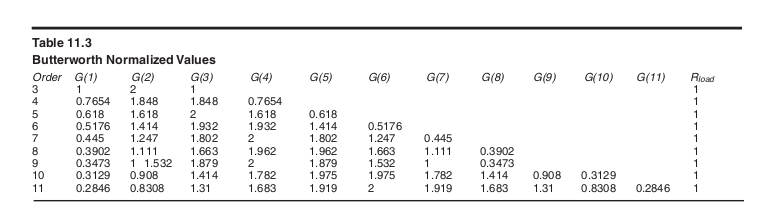
What do these tables represent? The normalized values tables represent component values necessary for a low-pass filter with a cutoff frequency of 1 radian/s, and for an 1 Ohm input impedance. That seems like a pretty worthless filter, but we will later extrapolate these numbers to find components values for our desired filter. Choosing the third-order line on the above table, we are given 4 numbers: G(1), G(2), and G(3).  . Before doing any math, let’s draw the architecture of our filter:
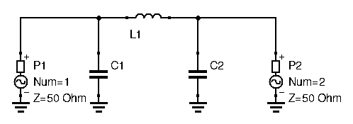
The first three values of the table, G(1), G(2), and G(3) correspond to component values from left to right. We’ve chosen a “Pi” architecture here, so the first value corresponds to a capacitance. Had we chosen a “Tee” architecture, the first value would have corresponded with an inductance.
Now that we have normalized component values, we need a way to scale them to our required frequency and output resistance. For low pass normalization, to get the actual component values the following equations are used:


With  being our cut-off frequency, and
  being the characteristic input resistance, 50 Ohms here. Applying these two formulas, we can find our actual component values:


And that’s it: we have our component values for our low pass Butterworth filter. For comparison, here is what QUCS’ filter design tool gives me for the same design constraints:
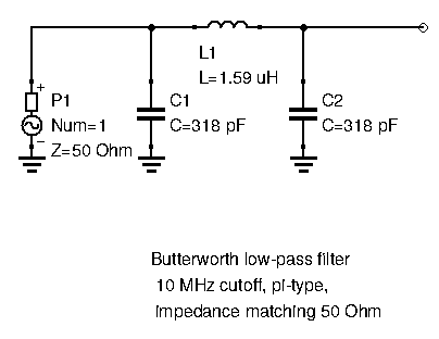
We obtain the exact same results. Now you know what goes inside your filter software.
There is one last step to take before we can actually build our filter. The values given by these equations (or our software) are impractical. We’ll have to use the closest standard capacitance available: here it would be 330pF. If we build our own inductor, we can get pretty close to the result, but we still will have some margin of error. At this point, we can test the filter with these new, standardized values and see if the response is close enough to what we initially wanted. Some tweaking might be necessary. Some filter design software will actually do this job for you and directly give you standard values to use. Handy.
High-Pass Filter Design
Let’s determine our design constraints. This time, we want a high-pass filter with a cut-off frequency of 5MHz, with a very steep rolloff, and atleast 70dB/decade of power attenuation. A Chebyshev filter would do nicely here. To have 70dB/decade power attenuation we would need a 4rth order filter at the least. When designing a Chebyshev filter, we also have to decide on the acceptable passband ripple. Here, we’re going to choose 0.5dB.
The first thing we need to do is find the table of normalized values for Chebyshev filters with 0.2dB ripple. Again, if you have an ARRL Handbook you should find some tables in the filters chapter. Otherwise, you can find them here. Here is the table from my copy of the Handbook:
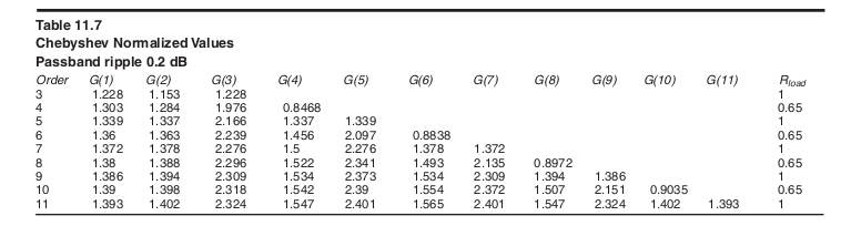
In this table, on the 4th order line, we have G(1), G(2), G(3), G(4), and . Here, isn’t equal to one, like it was with the Butterworth filter above. This means that the filter needs to feed a different resistance than its input resistance (which is usually 50 Ohms). Even ordered Chebyshev filters have different input and output terminations.
Let’s draw the architecture of the 4th order high pass filter:
To get the component values for this filter, a different set of denormalization equations is required:


This gives us the following component values:


Band-Pass Filter Design
The last filter example we will explore is the band-pass filter. Let’s first establish our design criteria:
- Wide bandpass filter with a center frequency of 15MHz, and a passband width of 3MHz
- Flat passband
- No steep rolloff needed
- Input resistance of 50 Ohms
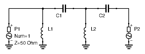
Again, a third-order Butterworth filter would work nicely here. First, let’s draw the filter’s architecture:
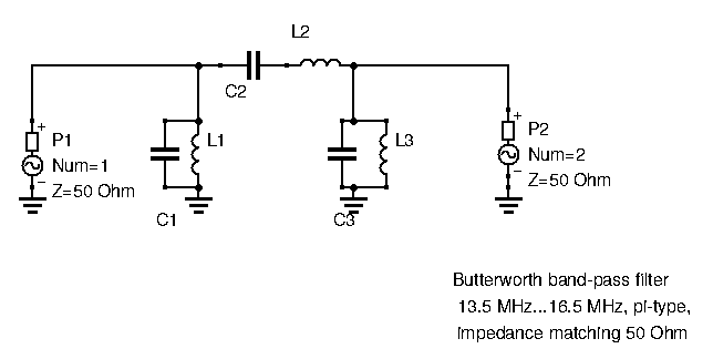
The following denormalization equations are used to get the actual component values:


With  being the width of the passband, and being the center frequency.
We can now calculate the values, using the same Butterworth normalized values table from the low-pass example:


And just to check our calculations against a proper filter design software, here is what QUCS’ filter design tool gives me for the same design constraints:
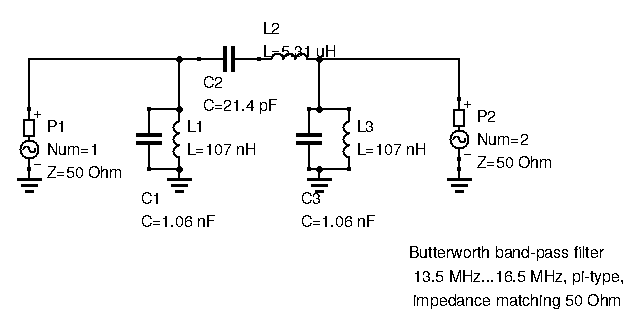
The values are identical.
Denormalization Equations
We could go into some more example, but I think you get the point. To design a filter with normalized tables, you need three things:
- The tables themselves, found in filter handbooks or the internet
- the filter topology, its architecture
- the denormalization equations
As you’ve no doubt noticed, the denormalization equations depend on the kind of filter you want: low-pass, high-pass, bandpass, and bandstop. However, they are the same for each filter family: the same equations will apply to Chebyshev, Butterworth, Cauer, and Bessel filters.
Let’s recap all the different denormalization equations you might need:
Low Pass Filters
being the cut-off frequency.
High Pass Filters
being the cut-off frequency.
Bandpass Filters
With being the center frequency, and being the passband width.
Bandstop Filters


With being the center frequency, and being the passband width.
Remember, for each one of this circuits, you can start with either the series elements, or the shunt elements. The equations don’t change: just apply them going from left to right.
Conclusion
Now you know how to manually design most kinds of LC ladder type filters. Even with all the tables and equations laid out, this is still slightly time-consuming. Which is why, once you’ve gone through the steps once or twice, I suggest you pick up a good filter design tool that will do all the tedious work for you. Most circuit simulation software will have a filter design tool somewhere in their menus. If you own a copy of the ARRL Handbook, a filter design software is often given in the attached CD-ROM. Otherwise, I suggest getting familiar with any circuit simulation software you like. I personally took a liking to QUCS. It’s open-source, relatively intuitive, and easy to use.