Mixers are a fundamental component in all RF communications equipment. They are required for nearly all modulation schemes, and have been present in radio in some or another since the beginning. Radio would not be possible without the existence of mixers. Despite their importance in radio equipment, many hams and experimenters are intimidated by them and don’t fully understand how they work. While you can actually design receiver and transceivers without knowing too much about the underlying theory of mixers simply by using trustworthy mixer chips (like the popular SBL-1 from Mini-Circuits), actually understanding the underlying principle behind mixers and the differences between different mixer types will allow you to make much more informed choices.
The Importance Of Mixers
While all the building blocks of a receiver are important, circuits in the front-end of the radio are much more sensitive with regards to their performance. A receiver can have multiple mixers, but there will always be one that is directly in contact with the RF signal, downconverting it to either baseband (audio range) in the case of Direct-Conversion receiver, or to an Intermediate Frequency in the case of a superheterodyne receiver. That mixer’s characteristics will heavily influence overall receiver performance. Indeed, keep in mind that RF signals have incredibly low power levels, and that translates itself to minutes amount of voltage present at the input of your first mixer (if no RF pre-amp is used). At those levels, even the smallest amount of spurious behavior or parasitic harmonics will heavily impact your receiver’s performance. This is why you will find many hams obsess over their front-end mixer’s performance: it is a key component that determines performance.
As we will soon learn in this article, not all mixers are created equal, and some are better suited than others for delicate RF work.
Essential Mixer Theory
Before diving into practical circuits and how they work, it’s important to first understand the underlying math behind mixers. A mixer has two inputs  and
and  and one output. Its output is the product of the first input signal and the second input signal:
  .
.
What does this mean in terms of frequency? Let and be two sine-waves of different frequencies:


In this case, a perfect mixer would output:
![\[ s_{out} = s_1 \timessf_2 = \sin(2 \pi f_1 t) \times \sin(2 \pi f_2 t) \]](http://modernhamguy.com/wp-content/ql-cache/quicklatex.com-3699f4eef1e09c4eb37a1f183c588bf6_l3.png "Rendered by QuickLaTeX.com")
Using the following trigonometric identity:
![\[ \sin(A)\sin(B) = \frac{1}{2} \times [\sin(A + B) - \sin(A-B)] \]](http://modernhamguy.com/wp-content/ql-cache/quicklatex.com-e5f248ca092563faf0b61b15368689c1_l3.png "Rendered by QuickLaTeX.com")
Our output signal is now:
![\[ s_{out} = \frac{1}{2} \times [\sin(2 \pi (f_1 +f_2) t - \sin(2 \pi (f_1 -f_2)t)] \]](http://modernhamguy.com/wp-content/ql-cache/quicklatex.com-4b5edb339e7b4c0c3bfe70832782980c_l3.png "Rendered by QuickLaTeX.com")
Our output signal has the sum frequency  and the difference frequency
  . A perfect mixer will only output these two frequencies. In general, we only need one of the two frequencies. Since they are far apart, the unwanted frequency can be easily filtered out.
Multiplying two signals shifts the frequency of one by the other.
When describing mixers, the following diagram is used:

The mixer’s two input ports are the RF (radio frequency) port, and the LO (local oscillator) port. The mixer’s output port is the IF (intermediate frequency) port. A perfect theoretical mixer wouldn’t differentiate between the RF and LO ports, but in practice this is not necessarily the case. The RF input is where we apply the low-power modulated RF signal. The front-end oscillator’s output is applied at the LO input.
Practical Mixers
Ideally, a mixer only outputs the sum and difference products, and nothing else. Unfortunately, this is never the case. In practice, mixers suffer from a variety of imperfections that degrade performance:
Port-to-Port Isolation
Port-to-port isolation is how much power from one port is fed to another. A mixer has three ports, and signals from either one of them can leak through to any other port. An ideal mixer will not have  and
and  in its output, but only
  and . Practical mixers however always have some leakage, and both and will be found in the output signal’s spectral diagram. The higher the port-to-port isolation, the less amount of leakage there is, and the less power these unwanted frequencies represent in the output signal. It is measured in dB.
Intermodulation Distortion (IMD)
When used in real conditions, the mixer RF input port will not always deal with just one single frequency signal. Often, numerous signals with close frequencies will be fed to the RF port. For example, let’s say we want to receive signal with frequency  , but there is another signal with frequency
  very close to . In this case, a real mixer will not only output
  and
and  , but it will also output third and higher order product.
Even-ordered products don’t matter much since their frequencies are very far from the wanted output frequencies, so they can be easily filtered out. However, the difference odd-ordered products fall very close to our wanted frequencies, and are thus much harder to get rid of. Odd-ordered products over 3 don’t usually matter much because their power level is very low and can be safely ignored. However, third-ordered products do matter. Their power level is high enough that it could significantly degrade overall receiver performance. Third-ordered products that will influence receiver performance are  and
and  . These are close enough to to be a problem.
A common figure of merit to determine how good a mixer is at rejecting these parasitic terms is the IP3 point: the third-order intercept point.
I’ve detailed the IP3 point in the amplifier characteristics post, but I’ll give a quick recap here:
When describing IMD behavior, we say that n-th order products are X-dB below the output power of the desired signal.
IMD increases with input power. In fact, n-th order products increase by n-dB for every 1dB of input power.
We can plot a graph with the power levels of both the desired output signals, and of the different IMD products:
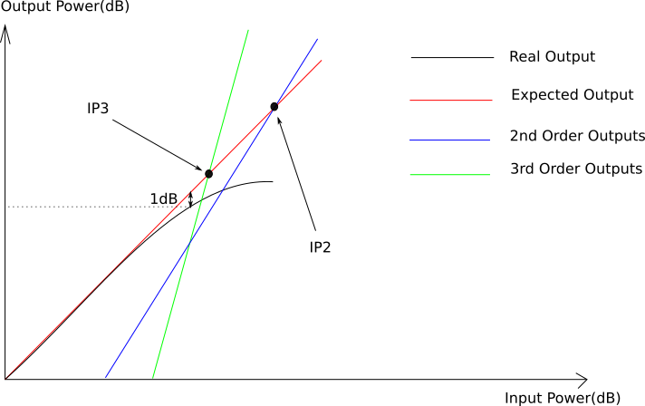
Extending the ideal output line and the third-order line gives us an the third-order intercept point. The same can be done for any order. For third-ordered products, this point is called the third-order intercept point,  . The higher this point is, the more resilient our mixer is to IMD, and the better the performance we can expect from a receiver.
Gain Compression
Just like for amplifiers, gain compression tells us how much input power we can apply at the RF input port before the output amplitude no longer follows linearly. This is illustrated by the diagram in the IMD subsection above. Often, the the 1-dB compression point is used: this is when output power deviates from expected power by 1 dB.
Some mixers do have gain, and thus the term gain compression is adequate. Many mixers don’t have gain. In this case, we use the term conversion compression.
Gain compression sets the upper limit on receivable RF power levels.
Dynamic Range
The dynamic range of a mixer determines the range of RF power levels it can handle. Its upper limit is set by its conversion (or gain) compression, while its lower limit is set by its noise figure.
Conversion Loss or Gain
When a passive mixer is used, the output power will always be less than the input RF power. This power loss, expressed in dB, is called the conversion loss. It is equal to the ratio of input power  to output power
  . It is always a positive quantity. The higher the conversion loss, the less efficient our mixer is.
Active mixers, on the other hand, can have gain. In this case, output power will be higher than input power. This power gain, in dB, is called the conversion gain. This time it is equal to the ratio of output power to input power . It is still a positive quantity.
Different Mixer Types
There are two different methods most commonly known to create a practical mixer: creating an analog mixer, or creating a switching mixer.
Analog mixers exploit non-linear components like diodes and transistors to simulate multiplication, whereas switching mixers repeatedly hash a signal to be able to have both sum and different products at their outputs.
Switching mixers offer better performance and are the ones most commonly used in today’s applications, but here we will cover both.
Analog Mixers
There are are few ways to create multiplication circuits with analog components. The first is to literally create a multiplication circuit with op-amps. This is possible using log, sum, and anti-log op-amp blocks. However, op-amps have terrible bandwidth, so this method is not used in RF.
There is another way to make analog mixer. First, we need to recognize that frequency multiplication is a non-linear operation. This means it can be achieved by exploiting non-linear components.
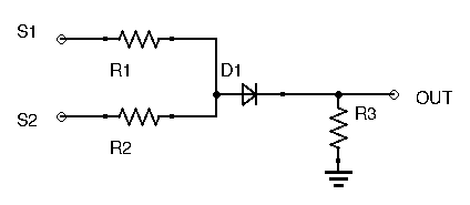
The simplest analog mixer uses a single non-linear component: a diode. We seldom think about a diode I-V characteristic, using it only to block current from going a certain way. However, a real diode doesn’t simply let current flow one way and blocks current flowing the other way. While this simplified approach is generally enough when the diode is very clearly in conduction or very clearly reverse-biased, near the diode voltage-drop, interesting things happen. In this area, the diode’s I-V characteristic is:
![\[ I = I_S (e^(\frac{q V_d}{kT}) -1) \]](http://modernhamguy.com/wp-content/ql-cache/quicklatex.com-53903114cad11c8ff46f4cc84de267d0_l3.png "Rendered by QuickLaTeX.com")
Where:
 is the saturation current
 is an electron’s charge
 is temperature (in K)
 is Boltzmann’s constant
 is voltage applied across the diode
 is current flowing through the diode
The constants don’t matter much to us here, so this equation can be simplified as:
![\[ I = I_S(e^(A V_d ) -1) \]](http://modernhamguy.com/wp-content/ql-cache/quicklatex.com-59db079b097ed9414e1ce8b786035597_l3.png "Rendered by QuickLaTeX.com")
Where  is a certain constant.
Using Taylor series approximation, we know that  . Therefore:
![\[ I \approx I_S \times (A V_d + \frac{(A V_d)^2}{2}) \]](http://modernhamguy.com/wp-content/ql-cache/quicklatex.com-8e9638a1a18ca10b29a635d9e2e21980_l3.png "Rendered by QuickLaTeX.com")
Now lets add two different voltages across the diode:  and
and  :
:
Ignoring the constants to simplify the equation, output current becomes:
![\[ (v_1 + v_2) + \frac{(v_1+v_2)^2}{2} = (v_1 + v_2) + \frac{v_1^2}{2} + \frac{v_2^2}{2} + v_1 \times v_2 \]](http://modernhamguy.com/wp-content/ql-cache/quicklatex.com-e41ff8c6ace6caf37113cd0fe731388e_l3.png "Rendered by QuickLaTeX.com")
Notice that last term gives us our product! Placing a resistor after the diode provides us with a voltage drop proportional to the above terms. Granted, we are also left with other unwanted terms. However, their frequencies are far away from our wanted products, so they can be easily filtered out.
This circuit was just to illustrate how we can exploit non-linear devices in order to simulate multiplication. Obviously it has glaring problems. Very careful biasing needs to be done, it is temperature dependent, and it has no port-to-port isolation just to name a few.
You will rarely find analog mixers in RF equipment. Nearly all mixers are now of the switching type.
Switching Mixers
The most popular method to achieve multiplication is high-speed switching. This means multiplying the input RF signal by +1/-1 at a certain frequency. It’s hard to instantly understand how this can actually produce sum and difference products in our output, so instead of going over the complicated math, I will simply show you some diagrams.
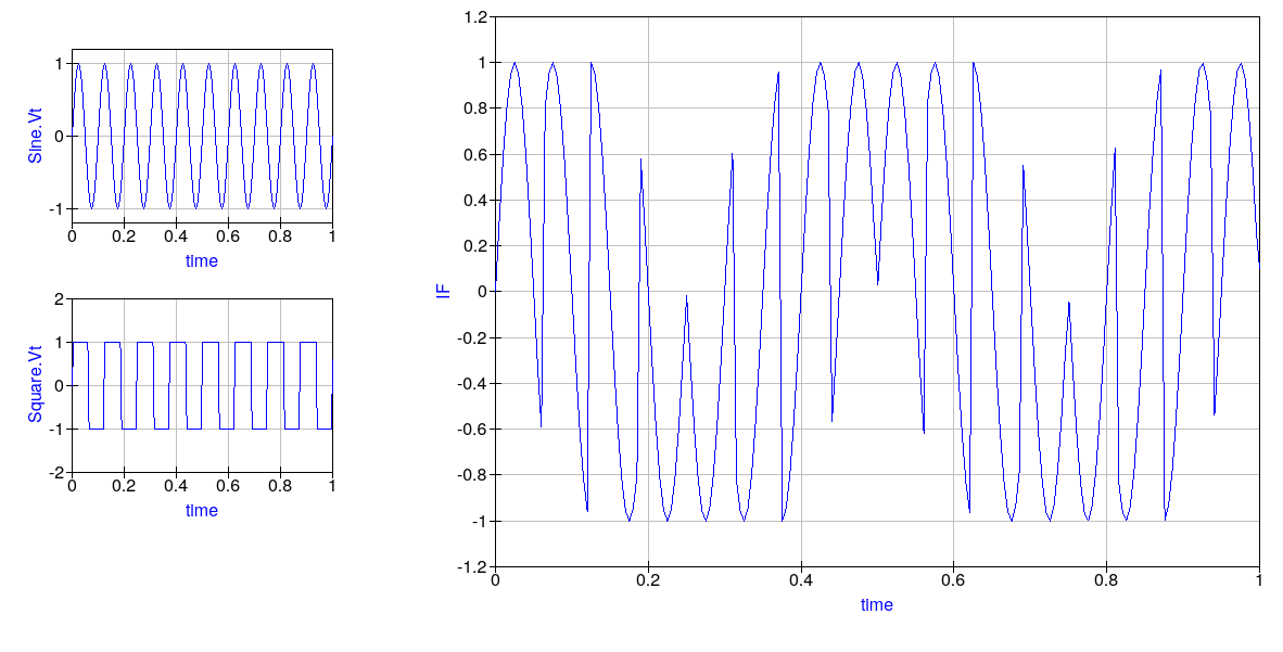
Above you will find the RF input sine wave signal, the LO input square wave, and the final output IF signal. Notice that when the LO signal is +1V, the IF output signal simply follows the RF input sine wave, but when the LO signal is -1V, the IF output is abruptly phase shifted 180° (inverted). This waveform has both the sum frequency  and the difference frequency
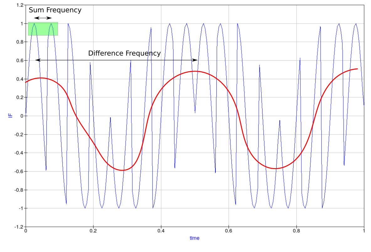
  . Can you spot them? To help you out, I’ve outlined both frequencies on the graph below:
Notice here that a square wave was used for the LO input, and not a sine wave. Since switching is the goal, it makes sense to use a square clock wave. Switching mixers would also work with sine waves, but usually designers prefer to stick to square waves. This often confuses experimenters. After all, square waves contain tons of harmonics – the Fourier transfer tells us that square waves have harmonics at every off multiple of its fundamental frequency. These harmonics can in turn mix with the input signals, causing heavy distortion. However, IMD products resulting from these harmonics are easily filtered out after the mixer. Furthermore, there is an advantage to using square waves over sine waves for the LO: using a square wave lowers the conversion loss of the mixer (around 2dB). Even without the lower conversion loss, using a sine wave for the LO to avoid harmonics usually won’t work. Switching mixers include diodes and transistors, non-linear components that will in any case create harmonics.
The Double-Balanced Mixer
There are many different types of switching mixers available, and covering all of them in this introductory article would be delusional. However, I think it’s a good idea to introduce you to the most popular switching mixer (at least for hams): the diode Double-Balance Mixer (DBM).
A mixer is considered either unbalanced, balanced, or double-balanced depending on whether or not its input frequencies are present at the output. If both input frequencies are present at the output, the mixer is unbalanced. If one of the two input frequencies (LO or RF) is present, the mixer is single-balanced. And if none of the two input frequencies are present, then the mixer is double-balanced.
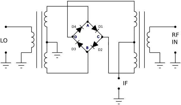
The above diagram is the schematic of a DBM. Assuming the LO signal is a square waveform, when the LO input is HIGH, diodes  and
and  (the right arm) conduct. Likewise, when the LO input is LOW, diodes
  and
and  (the left arm) conduct. Notice that points A and B are connected to ground via the transformer winding. Thus means that when the left arm conducts, point D is at ground, and when the right arm conducts, point C is grounded. We are alternating, at LO frequency, which end of the right hand transformer’s secondary winding is grounded. What this ends up doing is phase shifting by 180° (or inverting) the RF signal at each LO pulse. The switching action of the DBM is evident here.
For best performance, Schottky diodes are used for their low forward voltage and high switching speeds (RF-capable). Furthermore, the diodes need to have matching forward voltages. This can either be done by manually selecting matching diodes, or by simply using a monolithic diode bridge with guaranteed matching diodes. The diodes need to be heavily driven by the LO, and thus the power level of the LO should be much higher than the RF signal, to avoid the RF signal having any influence on diode conduction. LO levels 20dB over your expected RF input does the trick. If using packaged DBMs, such as the ones offered by Mini-Circuits, then be sure to drive them with the recommended LO power level indicated in the datasheet.
The many advantages of DBMs, along with their relative simplicity, makes them a component of choice for commercial and ham gear alike. They offer great port-to-port isolation and dynamic range, and being passive, don’t require any power source. Their conversion loss is reasonable (around 6dB is a common figure) and their distortion relatively low.
For many years, hams have loved using packaged DBMs (you’ll find the SBL-1 in many ham circuits) in their designs. However, it now seems that in many parts of the world, getting these popular chips is either impossible or very expensive: upwards of 20 dollars for a single chip. Considering the price and availability, building your own DBM can be better idea. A future article will be dedicated to this project.
Conclusion
Mixers are the heart of most communications gear, and are responsible for a good portion of a receiver’s performance. The sheer number of different mixers that exist and their apparent complexity deters many beginners from diving deeper into the subject. While we’ve only studied one of the more simple switching mixers out there, the DBM, know that the other mixer architectures you will find rely on the same switching action.