AMP II.6 – Amplifier Stability

Introduction

So far, everything we’ve learned about negative feedback seems to indicate that it is a great tool with little drawbacks. The only inconvenience we’ve actually talked about was a reduction in gain. Choosing a device, or a cascade of devices, that provide a big enough gain to start with solves this problem.

Unfortunately, negative feedback has a hidden cost to it that isn’t obvious at first: its negative influence on amplifier stability. This is the final big characteristic of feedback amplifiers we need to study to able to have a firm grasp on the basics of the subject.

When Negative Feedback Goes Positive

So, how does negative feedback decrease amplifier stability? Let’s look back at our block diagram:

As we’ve seen before, after the summing node the resulting signal feeds the amplifier $A$ and the feedback network $F$ , causing that signal to be multiplied by $AF$ . That resulting signal, the feedback signal, is then subtracted from the input, giving a smaller signal after the summing node. Depending on your amplifier, the way the feedback signal becomes negative is different: in a Common-Emitter amplifier, since the output is taken from the collector, the feedback signal is already 180° out of phase, making it negative relative to the input signal. In an op-amp, the feedback signal is applied to the negative input node of the amplifier, hence also creating negative feedback.

So knowing all this, where is the problem? Well, so far we’ve assumed that the output signal follows the input signal without any delays: at a certain time $t$ , if our input signal is $v_{in}(t)$ , then our output signal should be $v_{out}(t) = A \times v_{in}(t)$ . Unfortunately, while this is true for an ideal amplifier, all practical amplifiers will have delayed outputs: the output signal will always lag a little (or a lot, depending on some factors) behind the input signal, causing our output signal to look more like: $v_{out}(t) = A \times v_{in}(t + \phi)$ . Now, for small values $\phi$ , this won’t matter much. But what happens when delay increases? Let’s take a simple input test signal $v_{in}(t) = \sin(\omega t)$ , then our output signal is $v_{out}(t) = A\sin(\omega t + \phi)$ . What happens when $\phi = 180°$ , or $\pi$ radians?

$v_{out}(t) = A\sin(\omegat + \pi) = -A\sin(\omega t)$

After a delay of 180°, the sign of our output signal changes. The problem is we’ve already configured our amplifier so that our feedback signal would be negative. Having that signal change signs again will cause our feedback signal to become positive.

Once the output voltage is 180° out of phase with the input voltage, our negative feedback becomes positive feedback.

From Positive Feedback to Instability

It’s reasonable to think that the solution is simple: just avoid operating frequencies that induce more than 180° of lag. While in theory that would work, in practice a more thorough analysis is required.

First of all, even if our feedback becomes positive, it doesn’t necessarily mean that our amplifier becomes instantly unstable. For it to become unstable, the feedback loop has to increase the signal going through it constantly, until, after a certain amount of cycles, the output signal saturates. For the feedback loop to increase that signal, the loop gain $AF$ needs to be 1 or greater. If it is less than 1, the signal is dampened, and saturation will not occur.

So we now have our true definition of instability for our negative feedback amplifier: when phase shift is 180°, the loop gain $AF$ must be lower than 1.

This is also known as Barkhausen’s stability criterion.

Gain Margin and Phase Margin

In practice, when studying amplifier stability, we need to look at the Bode plot: a plot charting Gain vs. Frequency, and Phase vs. Frequency. In particular, we’d like to take study the bode plot of our entire negative feedback amplifier. Unfortunately, the only way to get a real Bode plot of your amplifier is by either creating the circuit and measuring gain and phase shit, or by using simulation software. Fortunately, in some cases it’s possible to get a good estimate of this plot using your active device’s datasheet: no wiring or simulation required.

Take a look at our high performance op-amp from the previous post: the TL081:

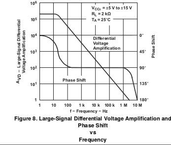
It’s the exact same chart as in the last post, and as you can see, we have both gain AND phase shift plotted against frequency. Notice that both axes are logarithmic: this is the standard way to graph a Bode plot: this allows us to have an easy conversion to dB on the y-axis, and a very large frequency range on the x-axis.

However, this Bode plot doesn’t give us the loop gain $AF$ . The datasheet doesn’t know what feedback network you are going to use. Instead, this Bode plot is for $A$ : it’s the open-loop gain of our op-amp. Since the graph is in log scale, we can use log arithmetic to draw the closed-loop Bode plot: $\log(AF) = log(A) + log(F)$ . If using an inverting amplifier op-amp setup, $F$ is simply the inverse of the gain. Gain being greater than 1, $F$ is smaller than 1, and thus $log(F)$ is negative. For a purely resistive feedback network, $F$ is constant throughout the frequency range. Thus, to find the gain loop Bode plot, we simply need to shift down the open-loop Bode plot by the constant value $F$ .

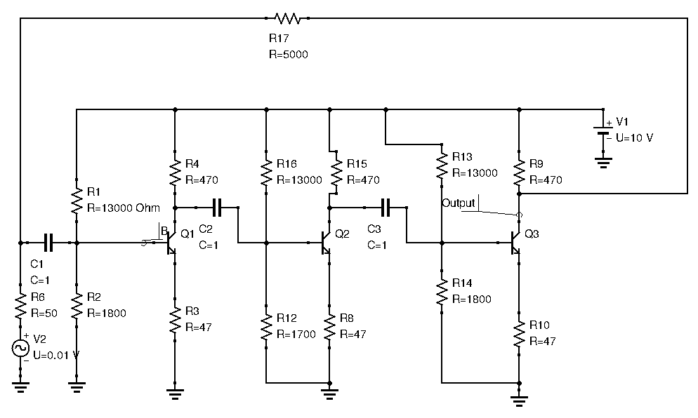
For a concrete example, let’s return to our 3 stage amplifier amp from previously, now with standardized resistor values:

This is the Bode plot the simulation software gives us:

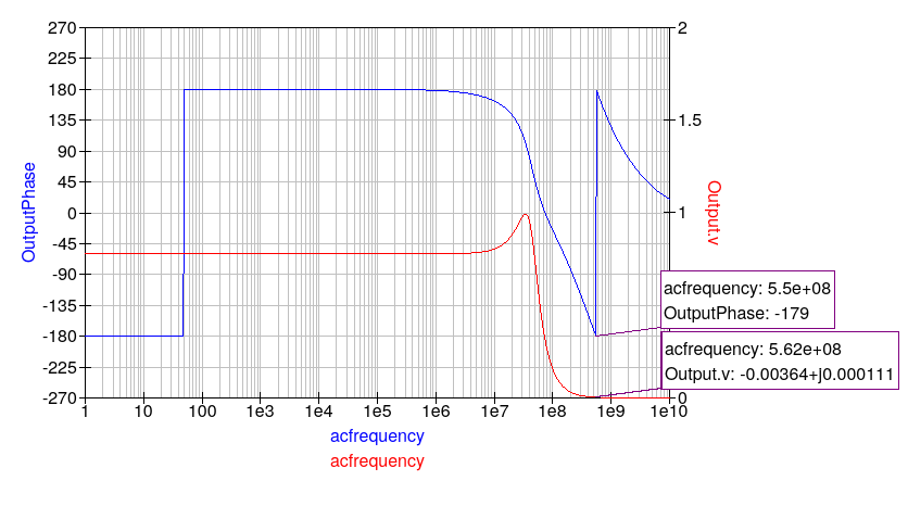
Don’t mind the phase shit from -180 to +180. QUCS’s phase function constrains values to ]-180°;+180°[. Here, consider phase shift is constant at -180° until the Megahertz range. Now, we said that approaching 180° phase shift for the output was dangerous for amplifiers, but keep in mind the above plot doesn’t include the fact that the output voltage is sampled at the collector, and thus already inverted (opposite sign as the input signal). Instead the graph represents that fact by phase shifting the output signal by 180° right from the beginning. Thus, on this particular graph we need to check if phase shift ever goes to 360°.

As seen above, at this critical phase shift, gain is near zero (input signal was 0.01V for comparison). Thus, the amplifier is theoretically stable.

In practice, just verifying the condition that at 180°, loop gain is less than unity isn’t enough to declare an amplifier stable. Depending on how close to unity that 180° gain is, you can guess that an amplifier is more or less stable, and one that is closer to unity will react differently than one who is much further away from the critical point. There are quite a few figures of merit and equations that describe amplifier stability, but one of the more simpler ones is one we can visually see directly on the Bode plot: the gain and phase margins.

As the name suggests, gain margin is how far below 0dB (0dB corresponds to unity gain: $\log(1) = 0$ ) our gain curve is at $f_{180}$ : the frequency at which phase shift is 180°. Phase margin is how far above 180° our phase curve is at $f_{1dB}$ : the frequency at which gain is 1dB.

To illustrate these two concepts, let’s take a look at the TL081 datasheet again, and more precisely the gain and phase curves:

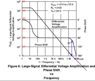
On the left y-axis, I converted the voltage gain to dB. Since the scale is logarithmic, this is easy to do. To find the phase margin, we need to locate the where the phase curve is when gain is 1dB, and compare that with 180°. This is illustrated by the blue arrow, and visually we find a phase margin or around 70°. To find the gain margin, we locate where the gain curve is when phase is 180°. The gain curve had to be extended to visually locate the gain margin. This is illustrated by the purple arrow, and visually we have a gain margin of around 4dB.

Whenever you have a Bode plot, this method will work.

For a more grounded explanation of gain and phase margin, think of it this way:

Phase margin determines if an amplifier will oscillate. The lower the phase margin, the more likely it is it will.
Gain margin determines how much the amplifier will oscillate, or “ring”

How Much Margin do you Need?

Now that we’ve defined what gain and phase margin were, the obvious question is, how much of it do we need? Even if theoretically, an amplifier with near zero gain and phase margin is stable, in practice this is a dangerous situation: many practical factors can reduce phase margin.

For this reason, a good rule of thumb is to design amplifiers with at least 45° of phase margin. This ensures that even if factors outside our control reduce the phase margin, our amplifier will remain stable.

The Influence of Gain and Phase Margin

Will gain and phase margin are critical values when studying an amplifier’s stability, they also have direct influence on an amplifier’s output response in the time-domain. A lower phase margin will cause the amplifier’s response to oscillate more when fed a step signal, and vice-versa. A low gain margin will cause the amplitude of these oscillations to be greater, and vice-versa.

Conclusion

Say we want to verify a negative feedback amplifier’s stability, let’s recap what we’ve learned:

Draw the Bode plot for the loop gain $AF$ of the amplifier. If you have access to the Bode plot of $A$ (thanks to the datasheet), and $F$ is not frequency dependent, no calculations are necessary and you need only shift down the open-loop Bode plot.
Find the Gain margin and Phase margin
Ensure that the phase margin is at least 45°

Stability is a fundamental characteristic of amplifier theory. When new (and old!) hams and experimenters design amplifiers, sometimes they end up with an oscillator instead. While tinkering around with different values of components will eventually give you a workable circuit (it’s the ham way after all), knowing the theory behind stability can give you a big advantage when designing new amplifiers.

You may still feel a tad confused about how to actually apply this in practice. Don’t worry, this post’s goal was to get you acquainted with instability and what you need to watch out for. Practical examples and ways to apply these new tools will come up shortly.