Introduction
So far we’ve talked about the effects of negative feedback on gain, input resistance, and output resistance. Those are all important characteristics, but if we want to design for RF, we need to take into account one more very important characteristic: bandwidth.
Bandwidth in Amplifiers
The most commonly used figure of merit concerning bandwidth is the 3-dB bandwidth. The 3-dB bandwidth is the frequency at which power gain is reduced by 3dB. A decrease in 3dB (a logarithmic scale) corresponds to a decrease in half the gain. So our 3-dB bandwidth is the frequency at which our power gain is reduced by half. In terms of voltage, the 3-dB bandwidth is the frequency at which our voltage gain is reduced by a factor of  . Why is that? Power can be expressed as:
![\[ P = \frac{V^2}{R}$ \]](http://modernhamguy.com/wp-content/ql-cache/quicklatex.com-5674cc37837c829da83c380ad9bc8d8c_l3.png "Rendered by QuickLaTeX.com")
So, voltage can be expressed as  . For a given
  , a reduction in half the power
  results in a reduction of of the voltage
  .
.
In general, when you see bandwidth in a spec sheet or elsewhere, they mean the 3dB bandwidth.
Since we will be designing circuits that will operate on high frequencies, bandwidth is of especially high importance to us. When designing a circuit for a particular frequency band, we need to ensure that this circuit can actually operate properly at such frequencies: its bandwidth needs to be bigger than our expected operating frequency.
Illustrating the Effects of Negative Feedback on Bandwidth
Now that we’ve given a brief definition of bandwidth, it’s time to explore how negative feedback affects it. To better illustrate this explanation, we’ll use a practical example, using the TL081 Operational Amplifier, a common, high-performance Op-Amp.
We will study Op-Amps in much greater detail in another section. For now though, just keep min mind Op-Amps have HUGE gain, and a nearly infinite input resistance.
When looking at the datasheet, we can spot the following voltage gain vs frequency graph:
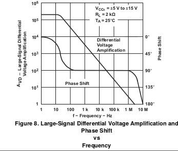
A very low frequencies, we can see that the (open-loop) gain of the Op-Amp is around  . Note here the graph is in log scale. Reading them can be a little confusing. A little trick I use to quickly get an approximate value when reading log scales without doing any calculation is to remember that dividing one decade into 2 equal parts gives me around 3dB (or 50%). So the halfway point from 10k to 100k would be approximately 30k.
Our initial voltage gain is indeed very big. However, if you look at the frequency response, we quickly see the drawbacks of our op-amp if it is used as is: gain is reduced by , to  , at around 50Hz. Hence, our bandwidth is a measly 50Hz. With this low a bandwidth no AC amplifier can be made with this op-amp as is.
By itself, this (and all other) op-amp makes a very poor amplifier: its bandwidth is poor and its frequency response is not stable at all. However, op-amps are not usually meant to be used as is (of course, there are still common use cases where they are used as such, but in these cases they are rarely used as linear amplifiers). Instead, op-amps love negative feedback. If you’ve studied any electronics after high school, then nearly all the material on op-amps was probably related to negative feedback in some way or another. The huge open-loop gain of op-amps makes it so that nearly all the time the loop gain is high enough for the closed loop gain to be entirely dependent on the feedback network  .
.
Let’s take a simple inverting op-amp amplifier configuration, as follows:
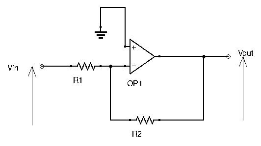
The closed loop gain of this circuit is  . Don’t worry if you don’t understand how to arrive to this result just yet, a whole section dedicated to op-amps is coming up soon.
Let’s see what happens to the bandwidth for different values of  and our loop gain
  :
:
 , = 0.1,
 , = 0.01,
 , = 0.001,
 , = 0.0001,
Now, let’s plot these different gain values on the voltage gain vs. frequency graph we found in the datasheet earlier:
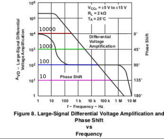
For each gain, we want to know the associated bandwidth (remember, bandwidth is when gain is reduced by a factor of  of its initial value at 0Hz, so it is NOT the frequency at which our closed loop gain curves crosses the original gain curve):
- For
 , bandwidth is approximately 700kHz.
 - For , bandwidth is approximately 70kHz.
- For , bandwidth is approximately 7kHz.
- For , bandwidth is approximately 700Hz.
These values are not exact, but should be close enough to the actual value. Reading a log scale without any measurements will of course lead to some margin of error.
As we can see, the lower our closed loop gain is, the higher the amount of feedback, and the higher our bandwidth is. Negative feedback increases bandwidth.
Since physics is so well put together, there is a relationship between closed loop gain and bandwidth:
![\[ BW_{cl} = (1 - G_{loop}) \times BW_0 \]](http://modernhamguy.com/wp-content/ql-cache/quicklatex.com-08de3918b7463873a27b392ed68593cb_l3.png "Rendered by QuickLaTeX.com")
Simple, right? With  being the new closed loop bandwidth, and
  being the open loop bandwidth. Again the magic quantity
  makes its appearance. Using the formula we obtain roughly similar values to the ones we graphically found above.
Another Way to Look at it
If this seems confusing to you, then perhaps seeing it in a different, more graphical way can help. Looking back at the initial Gain vs. Frequency curve, we can see that no matter what gain we ask of it, eventually the curve will go downhill with frequency. However, the frequency at which that point occurs depends on our gain. The higher our gain, the higher up on our graph we are, and thus the lower the frequency is at which gain starts to decrease, and vice versa.
Lower gain means more feedback. Lower gain also means we go lower on our graph. Pick a gain, draw a straight horizontal line and see where that line crosses our Gain vs. Frequency graph:
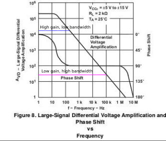
The frequency at that point is the maximum frequency the amplifier can tolerate without any decrease in gain.
As you can see, gain and bandwidth are trade-offs. More gain means lower bandwidth, and vice versa. For an amplifier, having stable gain throughout our range of operating frequencies is paramount. This means designing an amplifier with bandwidth greater than that of the largest frequency we will work with.
Conclusion
While feedback reduces gain by a factor of  , it increases bandwidth by the same amount. In the example above an op-amp was used: its absurdly high gain and readily available gain vs. frequency curves made it a great teaching tool. However, this holds true for any feedback amplifier, including those made from single transistors.