AMP I.6 – The Common Base Amplifier

Introduction

The common base amplifier is probably the most confusing and difficult of the three classical configurations to understand, especially for beginners. But with proper analysis techniques, it can be tamed.

When first introduced to BJTs, we are taught “if you put more current in the base, much more current will flow through the transistor”. So it’s very confusing for beginners when they see an amplifier where the input isn’t applied to the base. Indeed, in a common base amplifier, the input is actually applied at the emitter, will the output is sampled at the collector. Let’s see exactly how this circuit works.

Voltage Gain

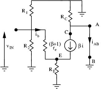
First, we need to draw out the small signal equivalent circuit:

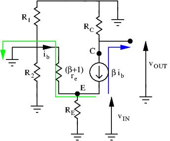
A KVL loop from ground to ground gives us:

$v_{IN} - v_{CE} - R_C \times i_C = 0$

With $v_{CE}$ being the voltage of the current source. Rearranging terms and replacing $i_C$ with $\beta \times i_B$ we have $v_{CE} = v_{in} - R_C \times \beta \times i_B$

Our goal is to express $v_{OUT}$ as a function of $v_{IN}$ . Lets see what we can do. Following the blue line:

$v_{OUT} = v_{IN} - v_{CE}$

Substituting v_{CE} with the expression found above, we obtain:

$v_{OUT} = v_{IN} - (v_{IN} - R_C \times \beta \times i_b)$

(1) $\begin{equation*} V_{OUT} = R_C \times \beta \times i_b \end{equation*}$

A second KVL loop (green line) gives us the following:

$v_{IN} -(\beta + 1) \times r_e \times i_b = 0$

Isolating i_b we get:

$i_b = \frac{v_{IN}}{(\beta + 1) \times r_e}$

Substituting i_b in equation (1) gives us:

$v_{OUT} = R_C \times \beta \times \frac{v_{IN}}{(\beta + 1) \times r_E}$

Since $\beta >> 1$ , we can safely make the approximation that $\beta +1 \approx \beta$ , and we obtain the following equation:

(2) $\begin{equation*} v_{OUT} = v_{IN} \times \frac{R_C}{r_E} \end{equation*}$

We have $A_v = \frac{v_{OUT}}{v_{IN}} = \frac{R_C}{r_E}$ . Since $R_C >> r_E$ , the CB amplifier has a high voltage gain.

Current Gain

We can’t use the same shortcut we used on the other two configurations. In the other configurations, input current was base current, and output current was either collector or emitter current. Thus, current gain was easily $\beta$ . Here, input is at the emitter, and output is at the collector. $v_{IN}$ forces a current into $R_E$ . This same current is found coursing through the transistor ( $i_C \approx i_E$ ). Academically, to find the current gain of a circuit, we short out the load and calculate the short circuit current, as shown on the above diagram. Shorting the load makes the AC signal ignore $R_C$ . All the current flows through the short. Thus, output current is the same is input current. Current gain is unity, or no current gain.

Input Resistance

We find the input resistance the usual way: by applying a test signal at the input and determining the test current.

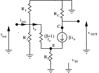
At the emitter node, test current flow to three branches: from the current source, to $R_E$ and to base. Thus, we have

$i_{TEST} = \beta \times i_b + i_{RE} + i_b$

Using Ohm’s law $i_b$ is easy to find:

$i_b = \frac{v_{TEST}}{(\beta + 1) \times r_E}$

Substituting for $i_b$ in i_{TEST}, and applying Ohm’s law for $i_b$ and $i_{RE}$ gives:

$i_{TEST} = \beta \times \frac{v_{TEST}}{(\beta + 1) \times r_E} +\frac{v_{TEST}}{R_E} + \frac{v_{TEST}}{(\beta + 1) \times r_e}$

$i_{TEST} =v_{TEST} \times [\frac{1}{r_e} +\frac{1}{R_E} +\frac{1}{(\beta +1) \times r_e}]$

We recognize a parallel resistance $[\frac{1}{r_e} +\frac{1}{R_E} +\frac{1}{(\beta +1) \times r_e}] = \frac{1}{r_e // R_E // (\beta +1)\times r_e}$ . Rearranging terms we obtain:

$v_{TEST} = (r_e // R_E // (\beta +1} \times r_e) \times i_{TEST}$

The input resistance is thus $R_{IN} = r_e // R_E // (\beta +1} \times r_e$ . When evaluating parallel resistances, take note of the lowest value. Here, it’s $r_e$ (tens of ohms generally). An equivalent parallel resistance has a lower value than any of its contributing resistors, so $R_{IN} < r_e$ . $R_{IN}$ is thus low.

Output Resistance

To simplify the process of determining the output resistance, let’s find the equivalent Thevenin circuit of our amplifier.

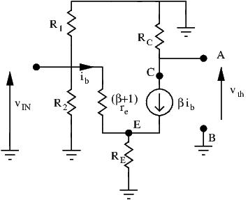
The open circuit voltage between A and B was already calculated previously when we derived the voltage gain. Here, $v_{AB} = -\frac{R_C}{r_e} \times v_{IN}$ . This is our Thevenin voltage.
Since we have both a dependent source $\beta \times i_b$ and an independent source $v_{IN}$ , we short AB to find the short circuit current $i_{AB}$ :

Since the short bypasses $R_C$ , the short circuit current is simply: $i_{AB} = \beta \times i_b$
A KVL loop from emitter to ground gives us the relationship between $i_b$ and $v_{IN}$ :

$V_{IN} -(\beta +1) \times r_e \times i_b = 0$

$i_b = \frac{v_{IN}}{(\beta +1) \times r_e}$

We can now find the final expression of $i_{AB}$ :

$i_{AB} = \beta \times \frac{v_{IN}}{(\beta +1) \times r_e} = \frac{v_{IN}}{r_e}$
We can now derive $R_{th}$ :
$R_{th} = \frac{v_{AB}}{i_{AB}} = \frac{R_C}{r_e} \times v_{IN} \times \frac{r_e}{v_{IN}} = R_C$
The CB amplifier can be simplified as :

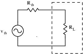
Quite trivially, we can now see that the output resistance $R_{OUT}$ of the amplifier is simply $R_{th} = R_C$ . This value can be moderately high.

Use Cases

Why would we want to use the CB amplifier? Its low input resistance comes in handy if we need to amplify signals that come from low resistance sources. It’s especially useful in audio circuits.

It also has its use in RF circuits. To understand why we’ll need a little more theory under our belt. We’ll explain why its so useful in the next chapter on the Miller effet.

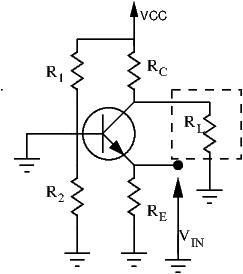
Design

Many people forget that in a CB configuration, the base must still be biased. Indeed, a stable voltage reference at the base must be applied, commonly through a voltage divider circuit.

Even more people are confused as to how this circuit even works, even after working through the equations. This circuit seems like it goes against the common logic of BJT: where input current at the base is amplified through C-E junction. But here, the base is “common” and no input signal is fed through it. So how can this amplifier work?

Well, with the voltage divider circuit, $V_B$ is constant. Yet $V_E$ changes with the input signal $V_{IN}$ . Thus, $V_{BE}$ is changing. There is a formula linking $V_{BE}$ and $I_C$ :

$I_C = I_S \times e^\frac{V_{BE}}{V \times T}$

This equation demonstrates the physics behind the transistor’s operation, but is seldom used for circuit design. Just know that chaning $V_{BE}$ causes $I_C$ to change with it. This is how the CB amplifier works. As $V_E$ goes lower, $V_{BE}$ increases and more current is sunk through the BE junction, lowering $V_C$ .

Conclusion

Let’s recap the fundamental characteristics of the Common Base amplifier:

$A_v = \frac{R_C}{r_e}$
$A_i$ \approx 1
$R_{IN} = r_e // R_E // (\beta +1} \times r_e \approx r_e</li> <li>$ R_{OUT} = R_C$