AMP I.14 – Amplifier Characteristics

Introduction

We’ve talked quite a lot about amplifiers so far. The different amplifier configurations, how to recognize them, and what each component is used for. By now analyzing familiar amplifier schemes shouldn’t prove too difficult. However, we haven’t really discussed the design part. The way I see it, a healthy education in practical electronics should go through 3 steps:

Understanding of the underlying basic electronics theory and classical circuits
Analysis and understanding of pre-built circuits. Before learning to design your own circuits you need to be able to understand the design decisions of others, down to the last component.
Design. Now using your own design criteria, you should aim to build your own circuits. Even with all your theoretical knowledge and your study of similar circuits, trial and error will still be necessary. But, your initial design should come close to your expectations.

But, if we want to design our own amplifiers in the best possible way, we need a few more tools at our disposal. So far, we’ve learned about voltage gain, current gain, and input and output resistances. However, we haven’t talked about what makes an amplifier “better” than another for a typical application. So far, our view of amplifiers is that they take an input signal, amplify it, and give us the same waveform, only bigger. Ideally, that’s what we want. Unfortunately, all amplifiers have limitations and imperfections. A few measurable variables are used to determine an amplifier’s performance. Let’s review them one by one, from easiest to understand, to the more complex topics.

Gain Compression

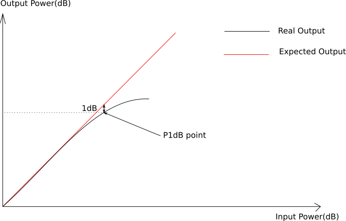
In an ideal amplifier, gain should be constant no matter what the input power is. Of course, in real life, there is a limit to the amount of power we can inject into our amplifier before the output deviates from what is expected. At a certain input power level the gain will start to decrease.

A common figure for evaluating this phenomenon is the 1-db compression point. It is the output power at which real gain deviates from expected gain by 1dB. This figure gives the most amount of power we can expect from our amplifier without having too much non-linearity.

Harmonic Distortion

An ideal amplifier is linear: its output is simply a linear function of its input. No frequencies other than the ones present at the input should find themselves at the output. Unfortunately, all amplifiers are non-linear to some extent, and at their output we will find multiples of the input frequencies in addition to the input frequencies. For example, if the input signal is a pure sine wave, then on an oscilloscope (time-domain), this would manifest itself as a distorted sine wave. On a spectrum analyzer (frequency domain), we would see energy on frequencies other than the fundamental.

Mathematically, we can measure this distortion with the THD – Total Harmonic Distortion ratio, defined by:

$THD = \frac{\sum_{n=1}^{\infty}F_n}{F_1}$

With $F_n$ being the power of the n-the harmonic, and $F_1$ being the power of the fundamental.

The lower the THD, the better.

Noise

Entire books can be dedicated to noise in electronic circuits. But for now, let’s try to keep it simple. We can identity two different kinds of noise: internal noise, and external noise.

External noise come from outside our electronic circuit, and include things like cosmic radiation, interference, and atmospheric noise. There isn’t much we can do about these noise sources, and we have to deal with them.

Internal noise, however, are generated within our circuit. This is something we can somewhat control! We won’t go too deep into the physical origins of noise. It’s important to know that it exists, and noise will indeed become a determining factor in receiver performance. For now, just keep in mind that a large part of the internal noise generated within the circuit is due to unavoidable random motion of electrons inside your circuit. This becomes more important the higher the temperature is.

It is possible to quantify noise with the noise factor F, or noise figure NF (in DB):

$F = \frac{N_{out}}{N_{in} G}$
$NF = 10log(F)$

With $N_{out}$ being the output noise power, $N_{in}$ being the input noise power, and G being the amplifier gain.

The noise figure NF can be found in a device’s datasheet. However, they should be taken with a grain of salt: the figure you will find in the datasheet often represents a best case scenario.

IMD: Intermodulation Distortion

This term will come up very often not just in amplifiers, but in nearly all the building blocks of radio. IMD characterizes how a circuit, amplifier or otherwise, behaves when 2 signals of different frequencies are applied at its input port.

In an amplifier, the desired outputs are the amplified signal frequencies $f_1$ and $f_2$ . However, for any circuit, whenever two or more different frequencies are applied to its input port, a phenomenon known as intermodulation occurs: not only will we find the input frequencies at the ouput, but we will also have the sum and difference of these frequencies. These frequencies are called IMD products, and depending on how the input frequencies are ‘mixed’, they can be 2nd, 3rd, or higher IMD products:

2nd order IMD products: $f_1 + f_2$ , $f_1 - f_2$
3rd order IMD products: $2f_1 - f_2$ , $2f_2 -f_1$ , $2f_1 + f_2$ , $2f_2 + f_1$
and so on…

When describing IMD behavior, we say that n-th order products are X-dB below the output power of the desired signal.

IMD increases with input power. In fact, n-th order products increase by n-dB for every 1dB of input power.

We can plot a graph with the power levels of both the desired output signals, and of the different IMD products:

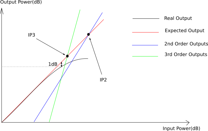
By extending the ideal output line and the x-order lines, interesting points become visible: the intersection between these two lines. This point is called an intercept point. This point has coordinates ( $IP_{XIN}, IP_{XOUT}$ ). More specifically, the third order intercept point is of particular interest to us, and is a widely use figure of merit for both amplifiers and mixers. Why is that? Well, 2nd order products are so far out of our range of wanted frequencies that they are easily filtered out and don’t affect performance much. Odd order-products over order 3 just don’t have enough power to truly bother us, even if they can come pretty close to our wanted range of frequencies.

Third order products however, are both inside the range of wanted frequencies (at least the difference products are. The sum products are out of range), so they are difficult to filter out, AND they also have enough power to noticeably affect performance. While the intercept point can be plotted on the chart, this point is fictional, and used only as a figure of merit. In reality, you will very likely never be able to input enough power to reach that point without overloading the circuit.

The higher our $IP_3$ is, the more resistant to IMD our amplifier is.

The most straightforward way to get $IP_3$ is to make a range of measurements and plot the above chart.

Conclusion

To be able to design a good amplifier, we must first know what characterizes a good amplifier. The following characteristics are all very important when considering amplifiers:

Gain Compression
Harmonic Distortion
Noise
Intermodulation Distortion, and especially third-order intercept point $IP_3$ .