The Problem with Open-Loop Design
So far, all the designs and configurations we have explored have been open-loop amplifiers. What is an open-loop amplifier? Simply said, it is an amplifier whose action is independent of its output. No matter what the output signal looks like, the amplifier is blind to it and just amplifies its input signal. Isn’t that what we want? Well the gain and bandwidth of open-loop amplifiers, also called feedforward amplifiers, are heavily dependent on the active device used: typically a transistor (JFET or BJT). The problem here is that not all transistors of the same type are identical. Take two 2N3904s (BJT NPN), and they will present slightly different characteristics, most notably in terms of gain and bandwidth. This is made clear when reading the datasheet. Notice that you don’t have a fixed value for most parameters, instead you have a range of values, with a minimum, maximum, and sometimes an expected value. This is true for all active semiconductors, and is especially pronounced in JFETs.
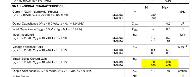
What this means is that, using the same schematic, two identical circuits can exhibit different behaviors. Granted, the differences may not be enormous, and for some applications it won’t matter. However, if we want precise control over our gain and overall circuit behavior, open-loop circuits won’t do. When using open-loop circuits, results are not reproducible.
A Solution to Semiconductor Variability
One way to fix this problem is to make it so our circuit’s behavior depends entirely on external circuitry instead of our active device’s parameters ( ,
,  ,
,  …).
…).
This exact problem was encountered many decades ago, in the early 20th century. The limiting factor of communications technology back then was the huge drift of gain in the active devices of the time: the vacuum tubes. A revolutionary concept which consisted in feeding a part of the output signal back into the input was introduced and solved this huge problem. As we’ll find out later, negative feedback increases stability, reproduce-ability, improves linearity, and increases bandwidth. All good things for radio circuits! If you want to learn more about how feedback was created, I highly suggest you look up Harold Stephen Black, the father of the field.
You will find feedback in nearly all fields of electronics, and it is a tool widely used by engineers and amateurs alike. Truly understanding feedback is like obtaining a superpower over the field of RF design. You cannot go very far in radio circuit design without understanding and applying negative feedback.
What’s the Difference?
While open-loop amplifiers were blind to their outputs, negative feedback amplifiers constantly receive information about the state of their output, and they strive to “correct” that output should it stray away from its intended value.
For a simple analogy, think of a car. Open loop control would be you solely focusing on the accelerator, without any regard for your speed. You may press the accelerator with the same strength on both a Fiat and a Ferrari, but your speed (your output) will definitely not be the same. Closed loop control, with negative feedback, would be you activating cruise control. No matter what car you wish to drive, you’ll always have the same speed.
What to Expect
When first tackling negative feedback, instructors almost always start with Operational Amplifier circuits. Op-Amps are also probably the first active device you will come across if you’re studying any kind of electronics after high school. I can understand their decision: with op-amps, feedback is almost trivial to exploit. Just one formula and you can tackle any feedback op-amp circuit. The problem with this approach is that even if understanding op-amp feedback circuit can come relatively quickly and easily, very often the student finds the skills don’t transfer to other active devices like BJTs and FETs. The reason for this is that many learn the necessary formulas for op-amp circuitry, but haven’t mastered the underlying general theory, or don’t know how to apply them to devices other than op-amps.
For this reason, the examples in this section will be heavily biased towards BJT applications, although some op-amp circuits will also be shown. The goal here is not to have learn by heart countless equations, but to understand the theory behind feedback, and memorize a few steps that will allow you to characterize any feedback circuit.
This section, AMP II, will consist of the following chapters:
- Introducing Feedback
- General Theory of Feedback Amplifiers
- Circuit Analysis of Feedback Amplifiers
- Determining the Loop Gain
- Input and Output Resistances of Feedback Amplifiers
- Ideal and Real Transfer Functions of Feedback Amplifiers
- Conclusion
Conclusion
We will dedicate many posts and chapters on negative feedback. This is a college level topic that can be very complicated. The math itself is far from trivial, and plenty of new techniques and tricks will be introduced. Don’t worry though, every step will be clearly explained, and we will slowly but surely dissect the rich field of negative feedback so you can both understand circuits who use it, and also use negative feedback in your own designs. While this topic is quite complicated, if you’re like me you’ll also find it incredibly fascinating!